Using the API

This tutorial walks through the API's capabilities, starting with a broad overview of your parks and narrowing to individual trail visualizations. By the end, you'll know how to query parks and trails, generate visualizations, build a 3D elevation profile for a specific trail, and use natural language search.

The tutorial assumes you've completed the Getting Started guide, run the full data collection pipeline, and have both Docker services running.

The examples below use curl with python3 -m json.tool for pretty-printed output. You can also paste the URLs directly into your browser, which is particularly useful for the visualization endpoints that return images and interactive HTML.

Tip: Don't want to set up locally? You can query the data endpoints on the live API demo, or explore the data through the Streamlit web app, which is a client of this API. In the examples below, replace http://localhost:8000 with https://seanangio-nps-hikes.onrender.com. Note that visualization endpoints and the natural language query endpoint (/query) are only available locally.

Orient yourself

First, confirm that the API is running and that the database is connected:

curl http://localhost:8000/health | python3 -m json.tool

You should see:

{
    "status": "healthy",
    "database": "connected"
}

The root endpoint lists all available endpoints:

curl http://localhost:8000/ | python3 -m json.tool

{
    "name": "NPS Trails API",
    "version": "1.1.0",
    "description": "Query National Park trail data from OpenStreetMap and The National Map",
    "documentation": {
        "swagger_ui": "/docs",
        "redoc": "/redoc",
        "openapi_json": "/openapi.json"
    },
    "endpoints": {
        "query": "/query",
        "parks": "/parks",
        "trails": "/trails",
        "hiked_points": "/trails/hiked-points",
        "stats": "/stats",
        "stats_parks": "/stats/parks",
        "park_summary": "/parks/{park_code}/summary",
        "us_static_park_map": "/parks/viz/us-static-park-map",
        "us_interactive_park_map": "/parks/viz/us-interactive-park-map",
        "static_map": "/parks/{park_code}/viz/static-map",
        "elevation_matrix": "/parks/{park_code}/viz/elevation-matrix",
        "trail_3d_viz": "/parks/{park_code}/trails/{trail_slug}/viz/3d",
        "health_check": "/health"
    }
}

Tip: For a full interactive reference, open http://localhost:8000/docs in your browser. The Swagger UI lets you try every endpoint, inspect request/response schemas, and experiment with query parameters.

Browse your parks

The /parks endpoint returns a park_count, a visited_count, and a parks array. Each park includes its 4-letter code, name, state, coordinates, and NPS URL.

curl http://localhost:8000/parks | python3 -m json.tool

To see only the parks from your visit log, add the visited filter:

curl "http://localhost:8000/parks?visited=true" | python3 -m json.tool

{
    "park_count": 3,
    "visited_count": 3,
    "parks": [
        {
            "park_code": "acad",
            "park_name": "Acadia",
            "full_name": "Acadia National Park",
            "designation": "National Park",
            "states": "ME",
            "latitude": 44.3386,
            "longitude": -68.2733,
            "url": "https://www.nps.gov/acad/index.htm",
            "visit_month": "Oct",
            "visit_year": 2024
        },
        ...
    ]
}

Visited parks include visit_month and visit_year from your visit log. Flip the filter to see your park bucket list:

curl "http://localhost:8000/parks?visited=false" | python3 -m json.tool

For richer responses, add description=true to include the full NPS description for each park:

curl "http://localhost:8000/parks?visited=true&description=true" | python3 -m json.tool

See the big picture

The API can serve map visualizations of all your parks. These endpoints return pre-generated images, so you need to generate them first. Run the US park map profiling module:

POSTGRES_HOST=localhost POSTGRES_PORT=5433 python profiling/orchestrator.py us_park_map

Now open the static map in your browser:

http://localhost:8000/parks/viz/us-static-park-map

This returns a PNG image showing all national parks on a US map with Alaska and Hawaii insets. Parks are color-coded by your visit log.

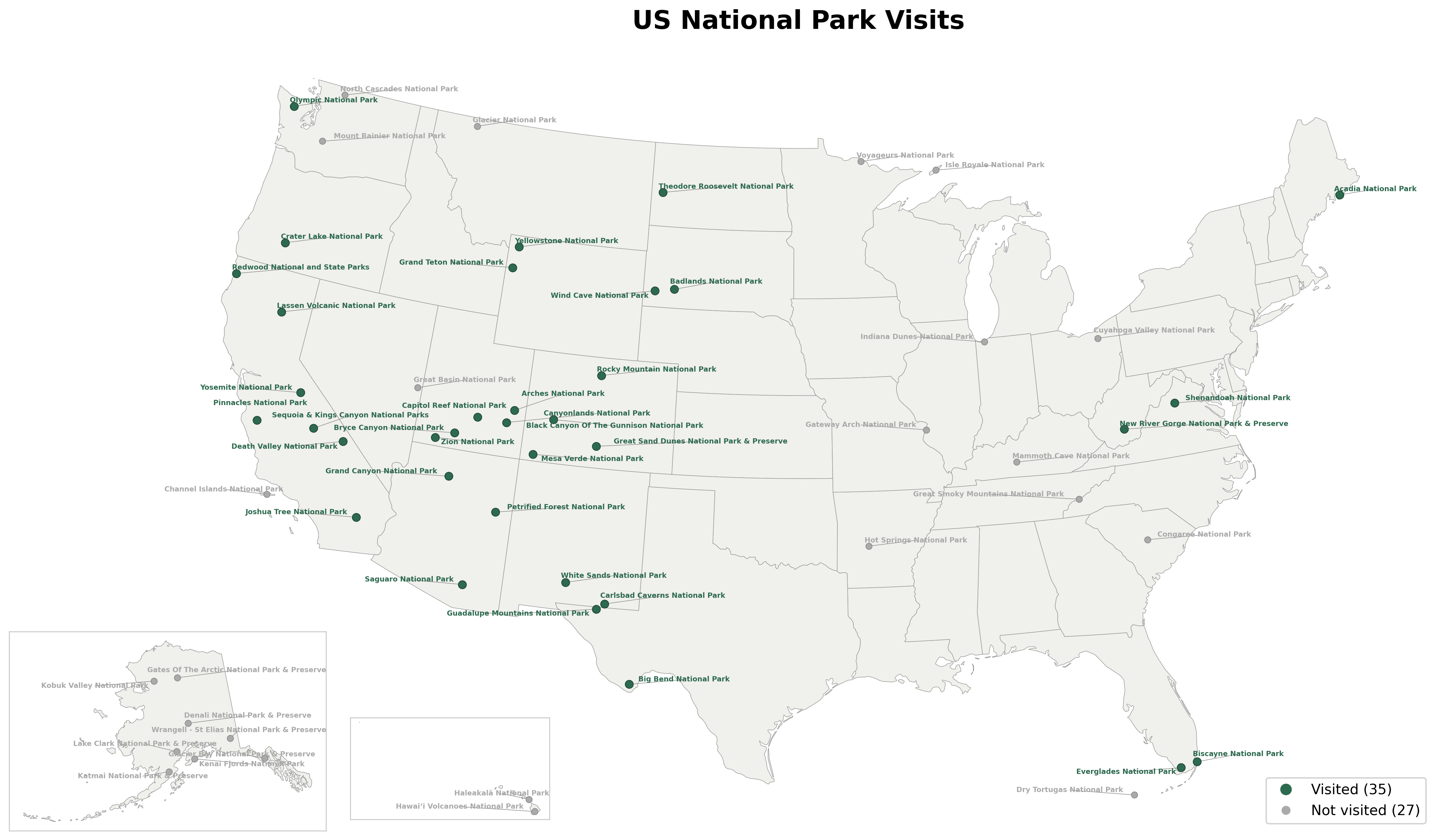
US park map showing visited and unvisited national parks

For an interactive version with hover tooltips and park boundaries, open:

http://localhost:8000/parks/viz/us-interactive-park-map

You'll get an HTML page with a zoomable Plotly map. Hover over any park to see its name, state, and visit status. You can zoom in to see (rough) park boundary outlines.

Park-level visualizations

The API also serves per-park trail maps and elevation charts. Generate them with:

POSTGRES_HOST=localhost POSTGRES_PORT=5433 python profiling/orchestrator.py visualization usgs_elevation_viz

Note: The visualization module generates static trail maps for every park with trail data. The usgs_elevation_viz module generates elevation matrices for parks with elevation data. Depending on how many parks have data, this may take a few minutes.

Static trail map

Open a trail map for a specific park using its 4-letter code:

http://localhost:8000/parks/acad/viz/static-map

The response is a PNG image showing the park boundary and all collected trails. Trails are color-coded by data source: blue for OpenStreetMap, orange for The National Map. Purple points mark hiking locations imported from your KML files.

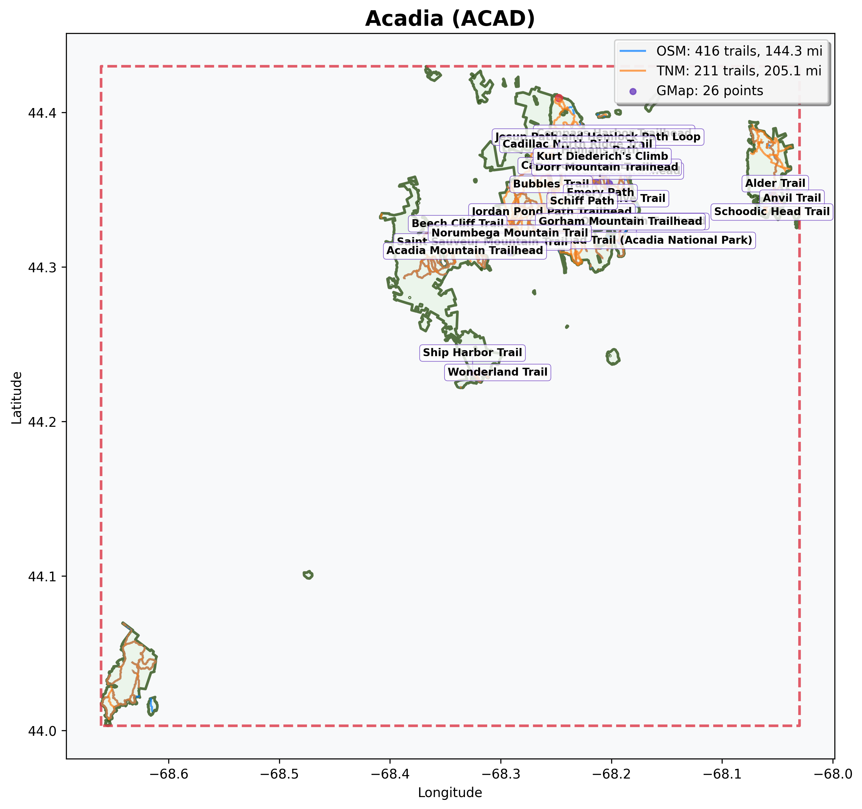
Acadia trail map showing OSM and TNM trails

Tip: Replace acad with any park code to see its trail map (for example, /parks/yose/viz/static-map for Yosemite).

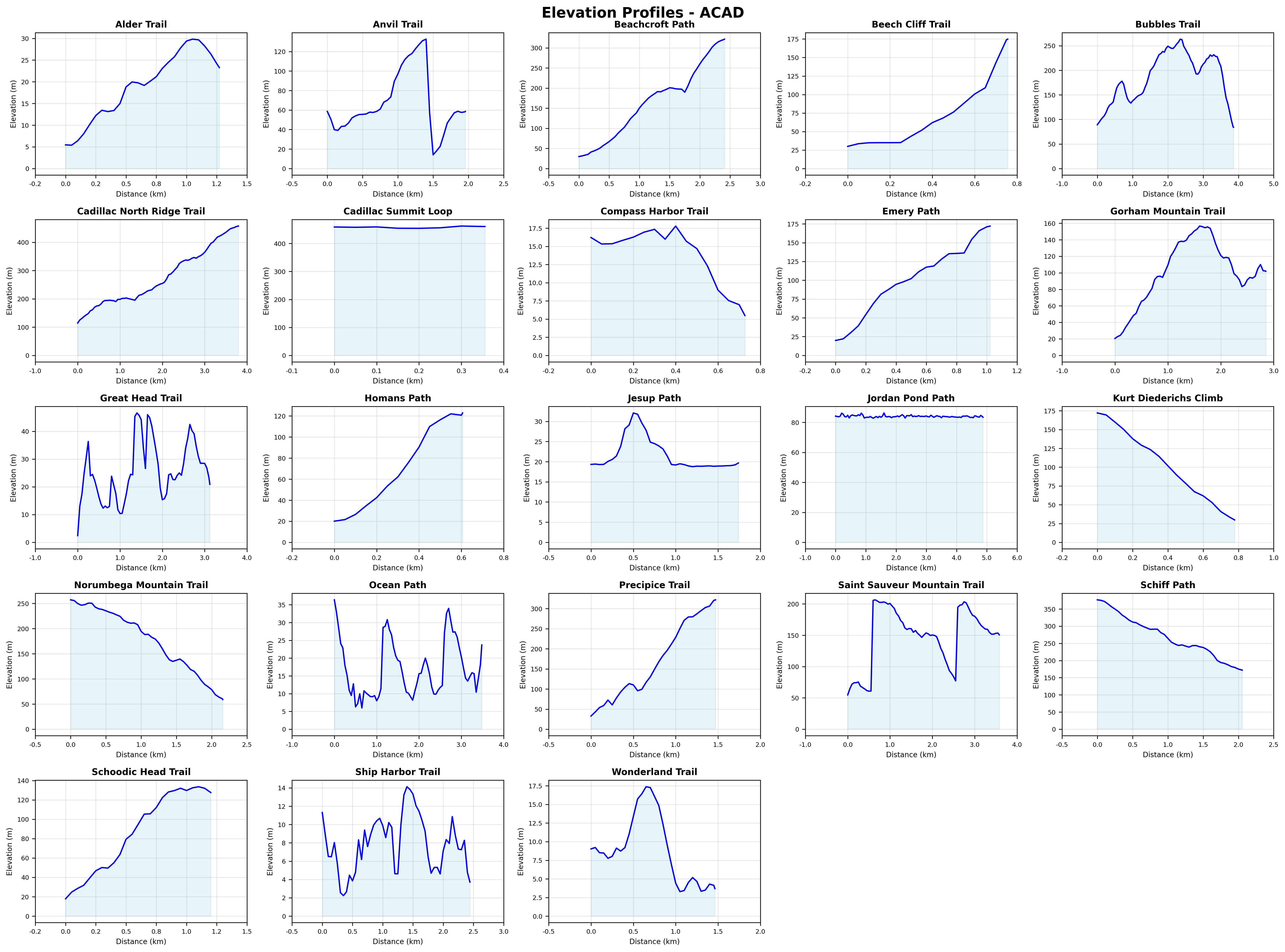
Elevation matrix

For parks where you have matched trails with elevation data, there's an elevation profile matrix:

http://localhost:8000/parks/acad/viz/elevation-matrix

This returns a PNG grid of elevation charts, one per matched trail. Each chart shows distance on the x-axis and elevation on the y-axis, giving you a quick visual comparison across trails.

Acadia elevation matrix showing elevation profiles for matched trails

Explore trails

The /trails endpoint returns trail data from both The National Map (TNM) and OpenStreetMap (OSM). Start by querying trails for a specific park:

curl "http://localhost:8000/trails?park_code=acad" | python3 -m json.tool

The response includes a trail_count, total_miles, a trails array, and pagination metadata. Each trail includes:

Field	Description
`trail_id`	Unique identifier (from TNM or OSM)
`trail_name`	Trail name
`source`	Data source (`TNM` or `OSM`)
`length_miles`	Trail length in miles
`hiked`	Whether you've hiked this trail (matched from your KML files)
`viz_3d_available`	Whether a 3D visualization can be generated
`viz_3d_slug`	URL slug for the 3D endpoint (if available)

When querying a single park, results are sorted by length (longest first). When querying across multiple parks, results are sorted by park code and trail name.

Note: The API deduplicates trails that appear in both data sources. When a TNM trail and an OSM trail in the same park share more than 70% name similarity, the API keeps the TNM version. This avoids double-counting while preferring the more detailed TNM data.

Pagination

The /trails endpoint returns paginated results to keep response sizes manageable. By default, you get 50 trails per page:

curl "http://localhost:8000/trails?park_code=yose" | python3 -m json.tool

The response includes pagination metadata:

{
    "trail_count": 50,
    "total_miles": 342.7,
    "trails": [...],
    "pagination": {
        "limit": 50,
        "offset": 0,
        "total_count": 127,
        "has_next": true,
        "has_prev": false
    }
}

The pagination object tells you: - limit: Items per page (50 by default) - offset: Number of items skipped (0 for first page) - total_count: Total trails matching your query - has_next: Whether there are more pages - has_prev: Whether there are previous pages

To get the next page, increase the offset:

curl "http://localhost:8000/trails?park_code=yose&limit=50&offset=50" | python3 -m json.tool

Or use page-based navigation (more intuitive):

# Page 1 (first 25 trails)
curl "http://localhost:8000/trails?park_code=yose&page=1&page_size=25" | python3 -m json.tool

# Page 2 (next 25 trails)
curl "http://localhost:8000/trails?park_code=yose&page=2&page_size=25" | python3 -m json.tool

You can request up to 1000 trails per page:

curl "http://localhost:8000/trails?limit=1000" | python3 -m json.tool

Tip: Use has_next and has_prev flags to build navigation controls in your app. Use total_count to show "Showing 1-50 of 127 trails" messages.

Filter by data source

Compare what each data source provides:

curl "http://localhost:8000/trails?park_code=acad&source=TNM" | python3 -m json.tool
curl "http://localhost:8000/trails?park_code=acad&source=OSM" | python3 -m json.tool

Filter by hiked status

See which trails you've hiked based on your KML data:

curl "http://localhost:8000/trails?hiked=true" | python3 -m json.tool

Or find trails you haven't hiked yet in a specific park:

curl "http://localhost:8000/trails?park_code=acad&hiked=false" | python3 -m json.tool

Filter by length

Find trails within a specific length range:

curl "http://localhost:8000/trails?min_length=5&max_length=15" | python3 -m json.tool

Filter by state

Query trails across all parks in a state:

curl "http://localhost:8000/trails?state=CA" | python3 -m json.tool

You can combine multiple states by repeating the parameter:

curl "http://localhost:8000/trails?state=CA&state=UT" | python3 -m json.tool

Note: State parameters surface state data as returned from the NPS API, rather than geographic validation. Keep this in mind when querying trails in parks that span multiple states (Yellowstone for example).

Check your stats

The /stats endpoint gives you aggregate numbers across all trails:

curl http://localhost:8000/stats | python3 -m json.tool

The response includes total trails, total miles, average trail length, parks and states visited, a source breakdown (TNM vs OSM), and the longest and shortest trails.

Filter to just the trails you've hiked for personal stats:

curl "http://localhost:8000/stats?hiked=true" | python3 -m json.tool

For a per-park breakdown sorted by trail count, use /stats/parks:

curl "http://localhost:8000/stats/parks" | python3 -m json.tool

Each entry shows the park's trail count, total miles, and average trail length. Add hiked=true to see only parks where you've hiked.

The 3D trail journey

The most detailed visualization in the API is an interactive 3D elevation profile for individual trails. Getting there takes a few steps because you need to discover which trails have elevation data and find their URL slugs.

Find trails with 3D data

Start by filtering for trails with 3D visualizations available:

curl "http://localhost:8000/trails?park_code=acad&viz_3d=true" | python3 -m json.tool

In the response, look for the viz_3d_slug field on each trail:

{
    "trail_count": 2,
    "total_miles": 5.8,
    "pagination": {
        "limit": 50,
        "offset": 0,
        "total_count": 2,
        "has_next": false,
        "has_prev": false
    },
    "trails": [
        {
            "trail_id": "123456",
            "trail_name": "Jordan Pond Path",
            "park_code": "acad",
            "source": "TNM",
            "length_miles": 3.4,
            "hiked": true,
            "viz_3d_available": true,
            "viz_3d_slug": "jordan_pond_path"
        },
        ...
    ]
}

The viz_3d_slug value is what you need for the next step.

Open the 3D visualization

Build the URL using the park code and trail slug, and open it in your browser:

http://localhost:8000/parks/acad/trails/jordan_pond_path/viz/3d

This opens an interactive 3D Plotly visualization. You can rotate, zoom, and pan the trail. The trail is color-coded by elevation using a terrain gradient (brown at lower elevations, cream in the middle, and blue-green at higher elevations). Hover over any point to see its distance along the trail and elevation.

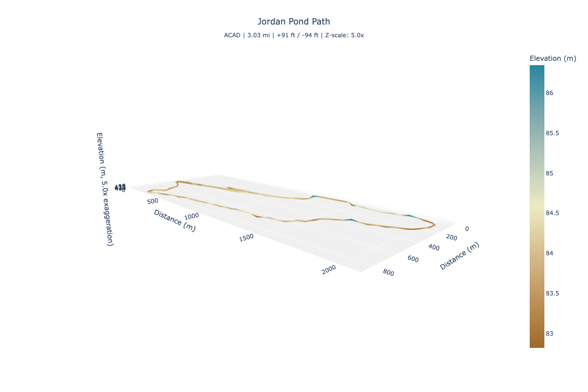
Interactive 3D trail visualization showing elevation profile

Adjust the vertical scale

By default, the z-axis is exaggerated by a factor of 5 to make elevation changes more visible. You can adjust this with the z_scale parameter (range: 1 to 20):

http://localhost:8000/parks/acad/trails/jordan_pond_path/viz/3d?z_scale=10

A higher value makes elevation changes more dramatic. A value of 1 shows true proportions, which can make trails appear nearly flat.

What makes a trail eligible

Not every trail has a 3D visualization. A trail needs elevation data, which requires this chain:

You added a hiking point near the trail in your KML files.
The trail matching step matched that point to a trail geometry.
The elevation collection step sampled points along the trail and queried the USGS for elevations.

This is why your KML files matter. They determine which trails get elevation data and 3D visualizations.

Note: Unlike the park maps and elevation matrices from the previous sections, 3D trail visualizations don't require the profiling step. The API generates them on-demand from the elevation data already in the database.

Combine and discover

All the filters on the /trails endpoint can be combined. Here are a few queries that answer real questions:

What long trails haven't I hiked in Utah?

curl "http://localhost:8000/trails?state=UT&hiked=false&min_length=5" | python3 -m json.tool

Which of my hiked trails have 3D visualizations?

curl "http://localhost:8000/trails?hiked=true&viz_3d=true" | python3 -m json.tool

From there, pick any trail with a viz_3d_slug and open its 3D visualization in your browser.

Tip: You can also use Python's requests library, the Swagger UI at /docs, or any HTTP client to query these endpoints.

Natural language queries

Instead of building query parameters by hand, you can ask questions in plain English using the /query endpoint. This requires Ollama running locally with a compatible model (see Prerequisites).

Start Ollama if it isn't already running:

ollama serve

Then ask a question:

curl -X POST http://localhost:8000/query \
  -H "Content-Type: application/json" \
  -d '{"query": "short hikes in Yosemite"}' | python3 -m json.tool

The response includes four fields:

Field	Description
`original_query`	Your question as submitted
`interpreted_as`	The structured parameters the LLM extracted (for example, `{"park_code": "yose", "max_length": 3}`)
`function_called`	Which function was used (for example, `search_trails`, `search_parks`, `search_stats`, `search_park_summary`)
`results`	The API results from the dispatched endpoint

The interpreted_as field is useful for debugging. If the results look wrong, check what parameters were extracted to understand how the LLM interpreted your question.

Example queries

# Trails you've hiked in Zion
curl -X POST http://localhost:8000/query \
  -H "Content-Type: application/json" \
  -d '{"query": "trails I have hiked in Zion"}' | python3 -m json.tool

# Parks you haven't visited
curl -X POST http://localhost:8000/query \
  -H "Content-Type: application/json" \
  -d '{"query": "which parks have I never visited?"}' | python3 -m json.tool

How it works

The endpoint uses a local LLM (via Ollama) to translate a question into structured parameters for the existing query functions (/trails, /parks, /stats, and /parks/{park_code}/summary). The LLM's only job is parameter extraction. It doesn't answer questions directly or generate SQL. Your data never leaves your machine.

The default model is llama3.1:8b (configurable via the OLLAMA_MODEL environment variable). You can swap models by changing the env var and pulling the new model with ollama pull <model_name>.

Note: The /query endpoint requires Ollama running on the host machine (not inside Docker). This allows the model to use Metal GPU acceleration on macOS for faster responses.